path = system.file("extdata", "case", "simple.ods", package = "floodam.cba")
case = import_case(path)
#> import Case from /usr/local/lib/R/site-library/floodam.cba/extdata/case/simple.ods
#>  ... done
dyke_sa = perform_sa(case, "dyke", n = 1000)
#> Model EAD: 5250
#> Model NPV: -41810
#> Registered S3 method overwritten by 'sensitivity':
#>   method    from
#>   print.src dplyr
#> Evaluating sa_model ...
#>  ... Elapsed time: 0.002012491 secs
#> Sensitivity analysis is performed using sensitivity::sobolmartinez
#> Evaluating sa_sobol ...
#>  ... Elapsed time: 0.4500911 secs
Uncertainty and sensitivity analysis: processing and outputs
2026-11-13
Note
Une version française de cet article est disponible : Analyse d’incertitude et de sensibilité : traitements et sorties.
Running the analysis (perform_sa())
perform_sa() executes the complete uncertainty and sensitivity analysis pipeline. It accepts either a Case object (with a project name) or a pre-built sa_input list from prepare_sa().
Key options controlling the estimation:
-
n: base sample size for Monte Carlo draws (defaults togetOption("floodam.cba")[["n_uncertainty"]]). Note that Sobol estimation evaluates model runs (where is the number of uncertain parameters); -
sobol_method: Sobol estimator from the sensitivity package (defaults to"sobolmartinez"). Settingsobol_method = "nominal"skips Monte Carlo and Sobol steps and evaluates only the nominal scenario; -
n_boot: number of bootstrap replicates for Sobol confidence intervals, controlled globally viagetOption("floodam.cba")[["n_boot"]](default100).
Structure of "cba_uncertainty" outputs
perform_sa() returns an object of class c("cba_uncertainty", "list") with four elements:
names(dyke_sa)
#> [1] "nominal" "u_a" "s_a" "input"-
nominal: parameter values and CBA indicators (benefit,npv) for the nominal scenario; -
u_a:data.framecontaining the Monte Carlo parameter draws together with simulatedbenefitandnpv; -
s_a: named list of two Sobol objects (npvandbenefit) produced in a single vectorized model pass; -
input: thesa_inputstructure used for the simulation.
Numeric summaries
dyke_sa[["nominal"]][c("benefit", "npv")]
#> [1] NA NA
summary(dyke_sa[["u_a"]][c("npv", "benefit")])
#>       npv             benefit
#>  Min.   :-236376   Min.   : 1562
#>  1st Qu.:-136497   1st Qu.: 3982
#>  Median : -93615   Median : 5215
#>  Mean   : -81053   Mean   : 5638
#>  3rd Qu.: -36602   3rd Qu.: 6945
#>  Max.   : 233416   Max.   :14970
prop_negative() computes the proportion of non-positive indicator values (e.g. probability that ), either globally or binned across a parameter’s range:
prop_negative(dyke_sa[["u_a"]][["npv"]], dyke_sa[["u_a"]][["npv"]])
#> v
#>    -236376    -184177    -131978     -79778     -27579      24620      76819
#> 1.00000000 1.00000000 1.00000000 1.00000000 1.00000000 0.03030303 0.00000000
#>     129018     181217     233416
#> 0.00000000 0.00000000 0.00000000
Diagnostic plots
The S3 plot() method for "cba_uncertainty" objects delegates to plot_sa(), providing unified access to all diagnostic visualizations.
Combined view (type = "both")
By default, plot() stacks the empirical distribution of the indicator and its Sobol sensitivity indices:
plot(dyke_sa)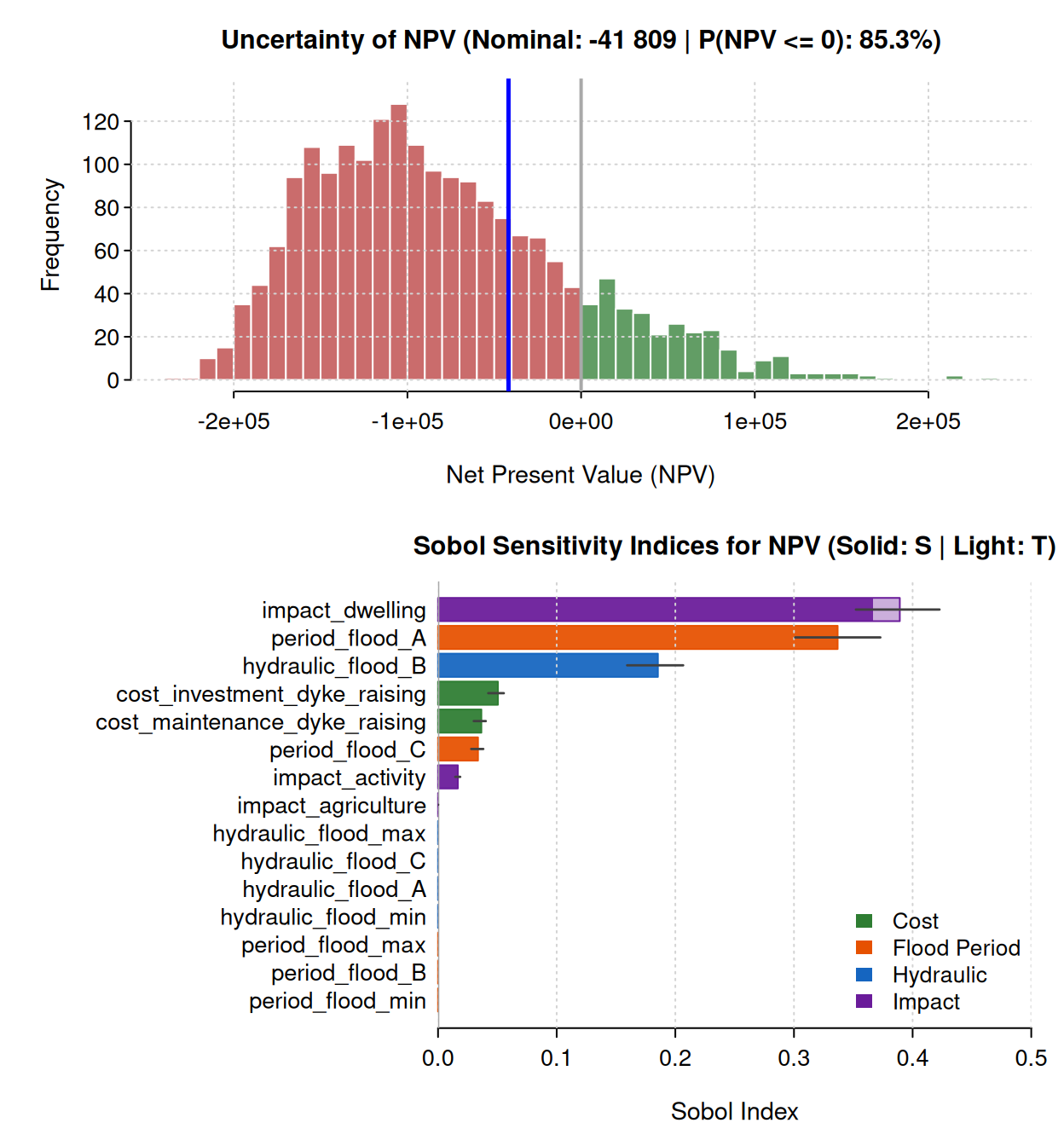
Uncertainty distribution (type = "uncertainty")
plot_uncertainty() (or plot(..., type = "uncertainty")) displays the histogram and/or density (distrib = c("hist", "density", "both")) of npv or benefit, highlighting the nominal value and the zero profitability threshold:
plot(dyke_sa, type = "uncertainty", indicator = "benefit")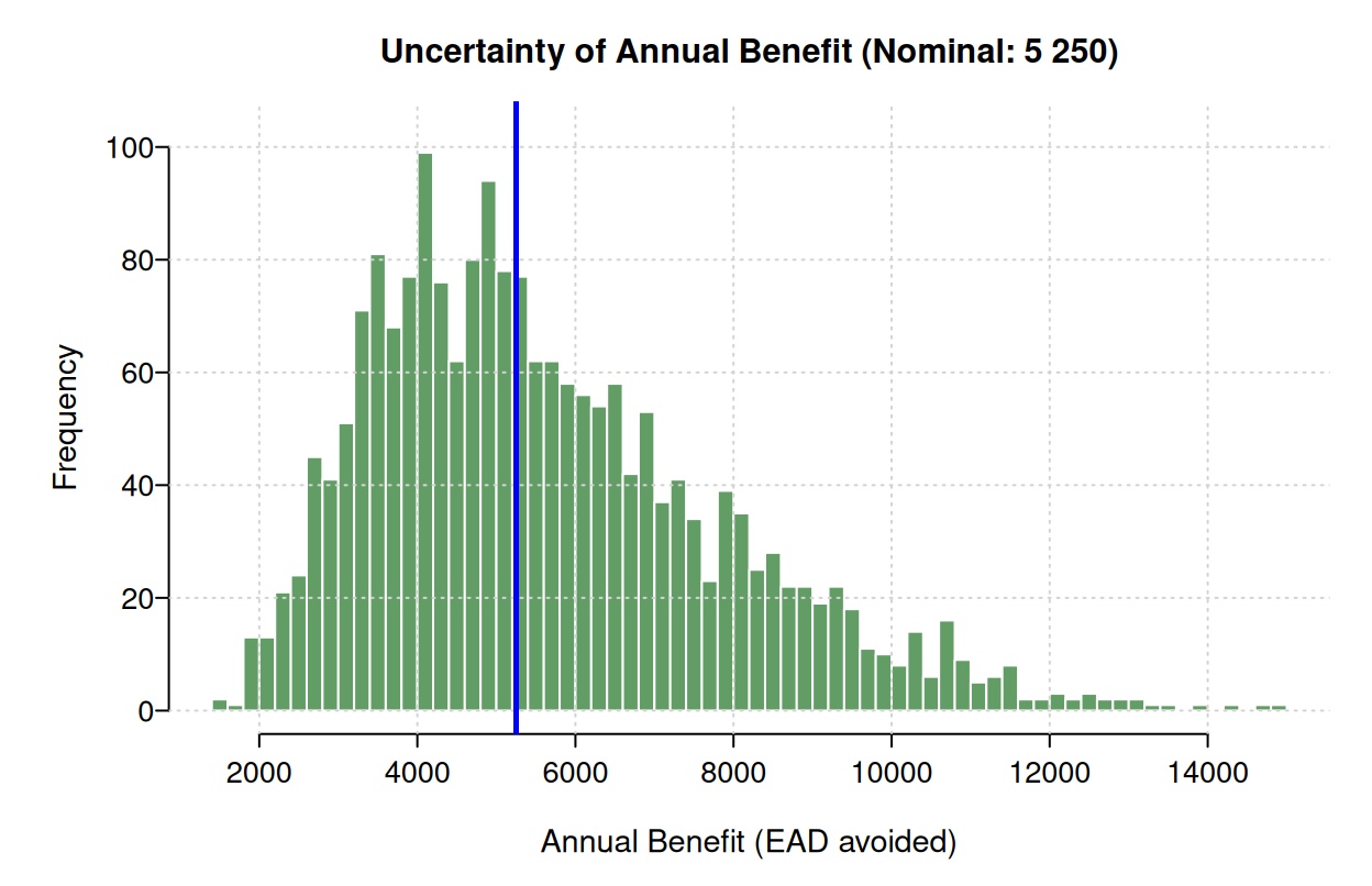
Sobol sensitivity indices (type = "sobol")
plot_sobol() (or plot(..., type = "sobol")) displays horizontal barplots of first-order () and/or total () Sobol indices (sobol_order = c("both", "total", "first")) with bootstrap confidence intervals, colored by parameter family (costs, return periods, hydraulic efficiency, stakes):
plot(dyke_sa, type = "sobol", sobol_order = "both")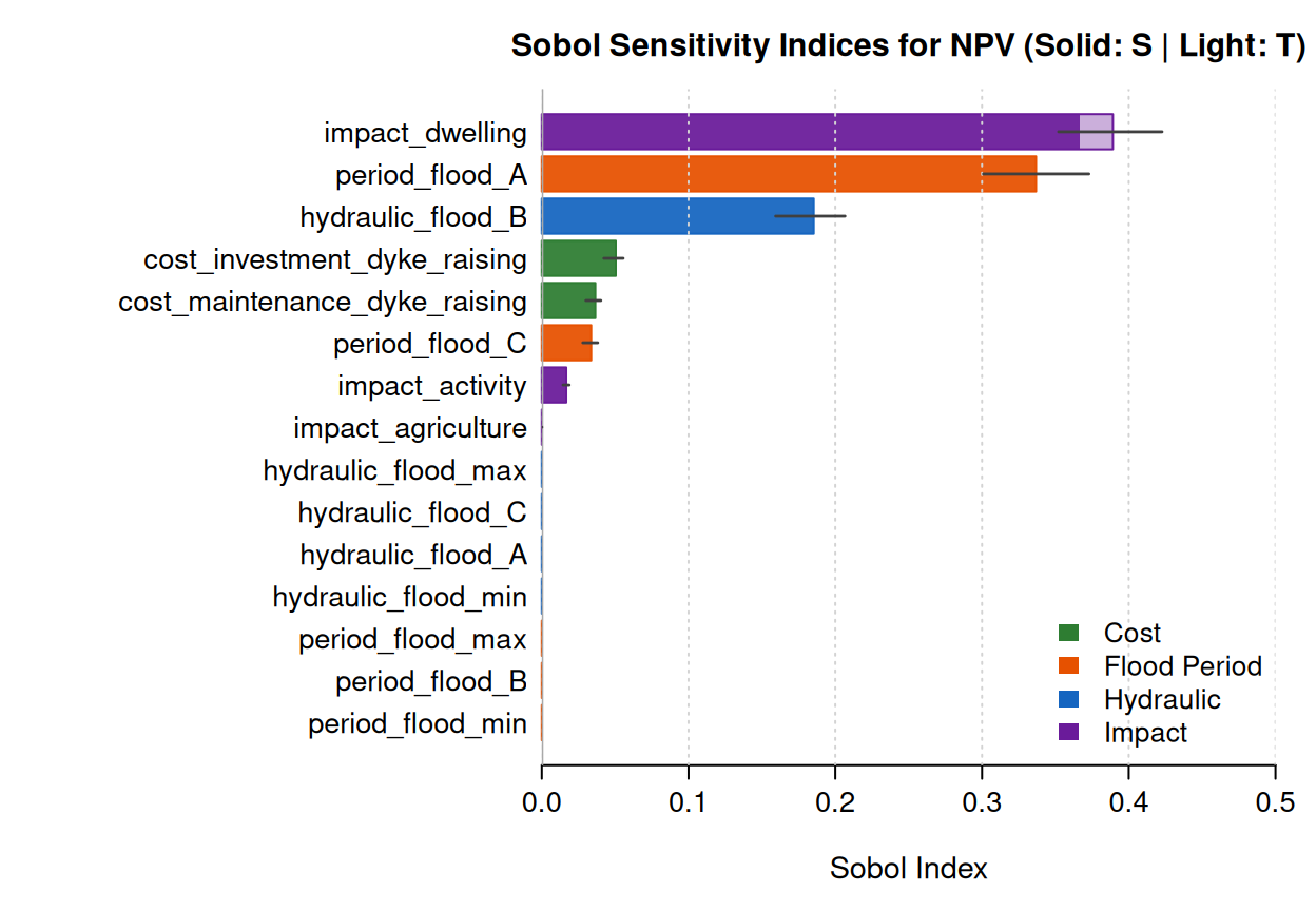
Triplet interaction matrix (type = "triplet")
plot_sa_triplet() (or plot(..., type = "triplet")) builds a 2x2 diagnostic crossing the 3 most influential parameters on npv (or benefit), showing their marginal distributions and the regions where the project becomes non-profitable:
plot(dyke_sa, type = "triplet")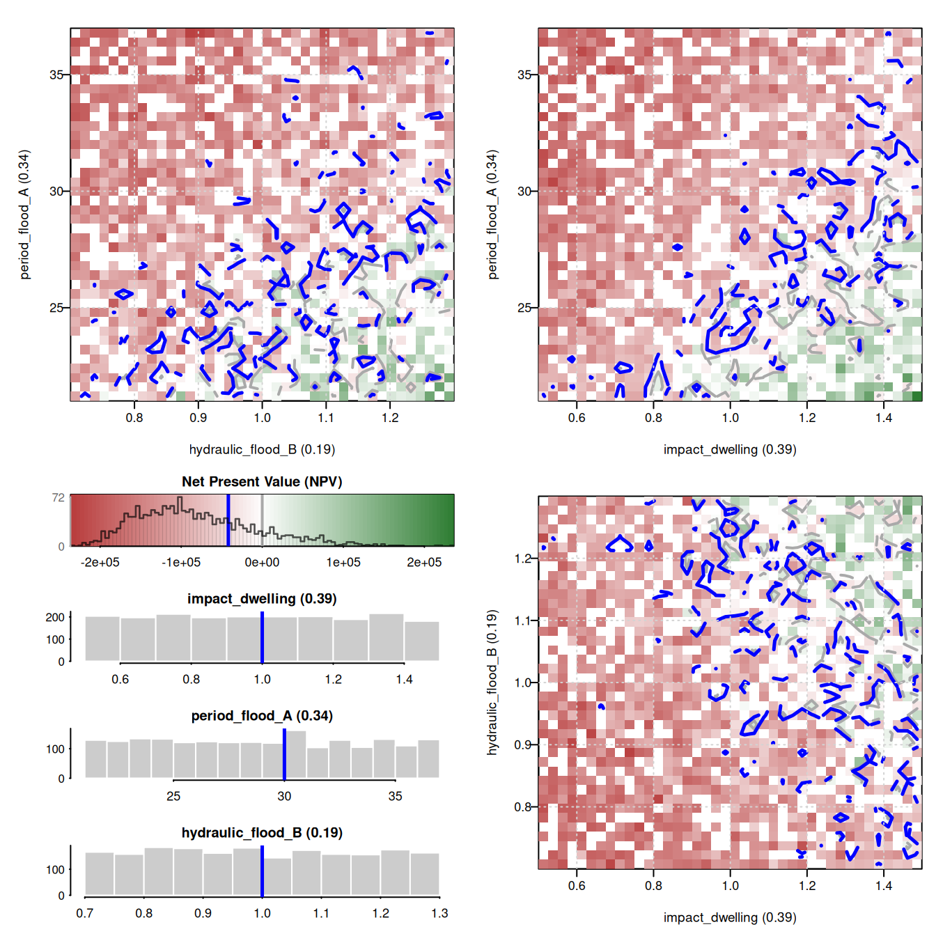
For customizing graphical output languages, report-ready A4 file exports, or package options (n_uncertainty, n_boot, sobol_method), see the dedicated articles Graphics and languages and Package options.