input_path = system.file(file.path("extdata", "case"), package = "floodam.cba")
Getting started
2026-11-13
Note
Une version française de cet article est disponible : Pour démarrer.
The library at a glance
floodam.cba is designed to carry out economic assessments of flood management projects. Based on an approach known as extended cost-benefit analysis, it enables the estimation of traditional cost-benefit analysis (CBA) measures, supplemented by additional indicators relating to aspects not necessarily included in the monetisation of project benefits or costs.
The impacts of projects on flooding are assessed according to the avoided damage principle, whereby avoided damage is defined as the difference between the impacts in the baseline scenario (without the project under assessment) and the impacts in the project scenario. It therefore enables the estimation of the benefits or costs of improvements or deteriorations in a territory’s exposure to flooding using different flood scenarios in both the baseline and project scenarios.
Other project impacts not directly attributable to a change in the area’s flood exposure are also considered. These impacts are analysed using a framework of actions, the implementation of which entails ‘one-off’ impacts during the implementation period and ‘deferred’ impacts that take effect once the action is completed and persist over time. The ‘one-off’ impacts include various investment costs (works, studies, easements, etc.). The ‘deferred’ impacts include maintenance costs, environmental impacts and any co-benefits expected from the project.
floodam.cba is particularly well-suited to applying the French government’s recommended method for the economic assessment of flood management projects. Its application in other contexts does not require significant adaptation.
This vignette provides a high-level description of the overall workflow you will use with floodam.cba. The specifics of some of the steps in this workflow are covered in separate vignettes.
Basic workflow
The process starts by providing the necessary input data on the situation before and after the project you want to analyse (i.e. the baseline and project scenarios, or hereafter cases for short). To make things easier and help you to learn how to use the library, floodam.cba is shipped with illustrative cases. The cases are available in your library’s installation folder, so just ask R to locate them:
Now let us load one of the cases available:
library(floodam.cba)
case = import_case(file.path(input_path, "complete.ods"))
#> import Case from /usr/local/lib/R/site-library/floodam.cba/extdata/case/complete.ods
#>  ... done
The import_case() function returns a S4 object of a new Case class defined by the library.
To process the case object and obtain a synthesis of indicators, we use the compute_synthesis() function, specifying the type of case:
case_ind = compute_synthesis(case)The compute_synthesis() function returns a matrix where rows represent the different indicators calculated by floodam.cba while columns represent the different projects proposed:
| complete | reinforcement | |
|---|---|---|
| npv | -1620.1569447 | 3987.8061188 |
| bcr | 0.7951837 | 3.2590387 |
| h_min | Inf | 12.0000000 |
| cost_hab | Inf | -Inf |
| cost_emp | Inf | -Inf |
| aad_pos | 178.5016342 | 74.3467025 |
| aad_neg | -136.0445764 | -18.5866756 |
| dam_eff | 0.0409014 | 0.0537170 |
| hab_eff | NA | NA |
| emp_eff | NA | NA |
| aadd | 46.2988617 | 62.7122250 |
| aad_ori | 1038.0333333 | 1038.0333333 |
| aad_fin | 991.7344717 | 975.3211083 |
| aadd_eff | 0.0446025 | 0.0604145 |
| aah_ori | NA | NA |
| aah_fin | NA | NA |
| aadh_eff | NA | NA |
| aae_ori | NA | NA |
| aae_fin | NA | NA |
| aade_eff | NA | NA |
Project calendar
You can inspect the annual evolution of states of nature for a project using plot_calendar_state():
plot_calendar_state(case, project = "complete", legend = "inline")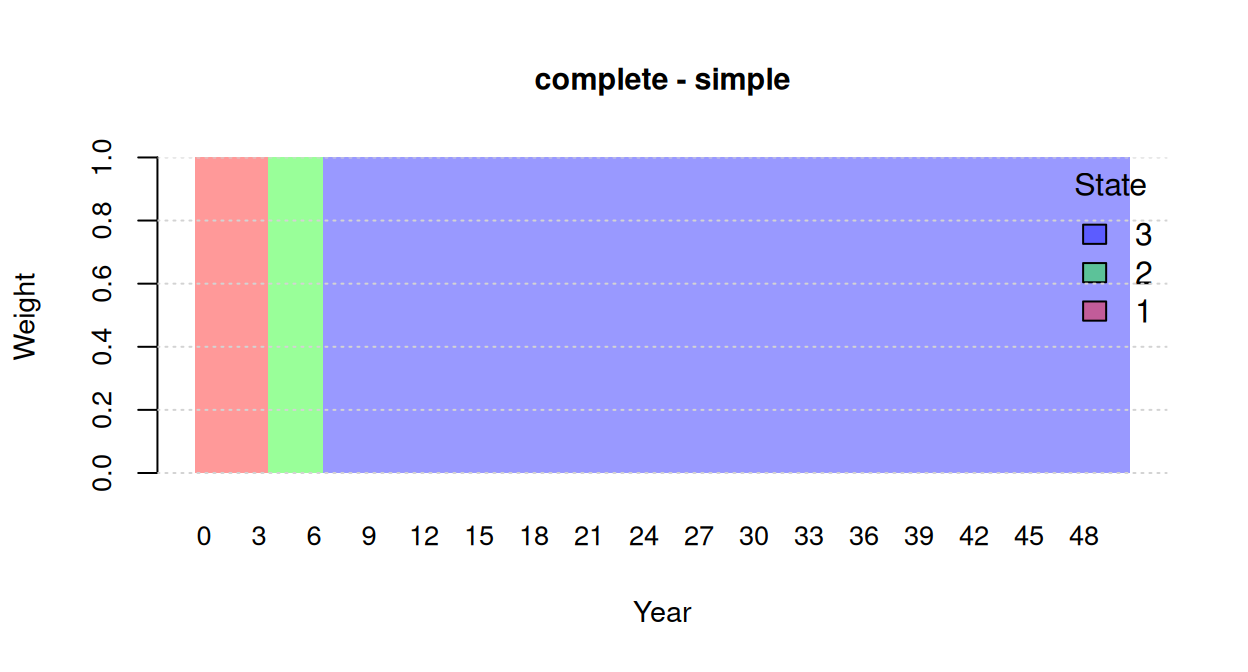
Uncertainty and sensitivity analysis
Finally, perform_sa() runs a Monte Carlo uncertainty analysis and a global Sobol sensitivity analysis on the project’s key parameters (costs, flood return periods, hydraulic efficiency, and damage estimations):
set.seed(123)
sa_complete = perform_sa(case, project = "complete", n = 1000)
#> Model EAD: 40.97
#> Model NPV: -1792
#> Registered S3 method overwritten by 'sensitivity':
#>   method    from
#>   print.src dplyr
#> Evaluating sa_model ...
#>  ... Elapsed time: 0.001924276 secs
#> Sensitivity analysis is performed using sensitivity::sobolmartinez
#> Evaluating sa_sobol ...
#>  ... Elapsed time: 0.3805578 secs
summary(sa_complete[["u_a"]][c("npv", "benefit")])
#>       npv             benefit
#>  Min.   :-9356.6   Min.   :-133.4784
#>  1st Qu.:-3877.6   1st Qu.:   0.7744
#>  Median :-2534.7   Median :  42.1221
#>  Mean   :-2471.6   Mean   :  43.2445
#>  3rd Qu.: -912.1   3rd Qu.:  86.2875
#>  Max.   : 4416.3   Max.   : 242.2300
The resulting "cba_uncertainty" object can be explored directly with plot() (combined uncertainty distribution and Sobol indices) or with the 2x2 triplet diagnostic (type = "triplet"):
plot(sa_complete)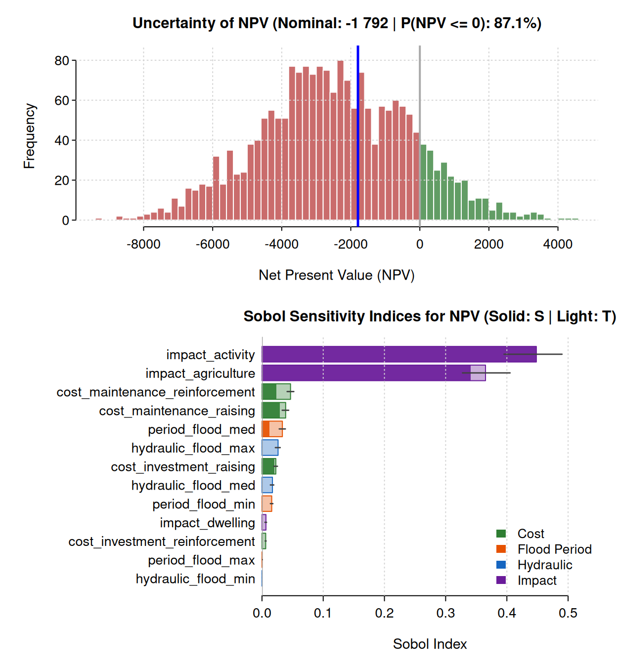
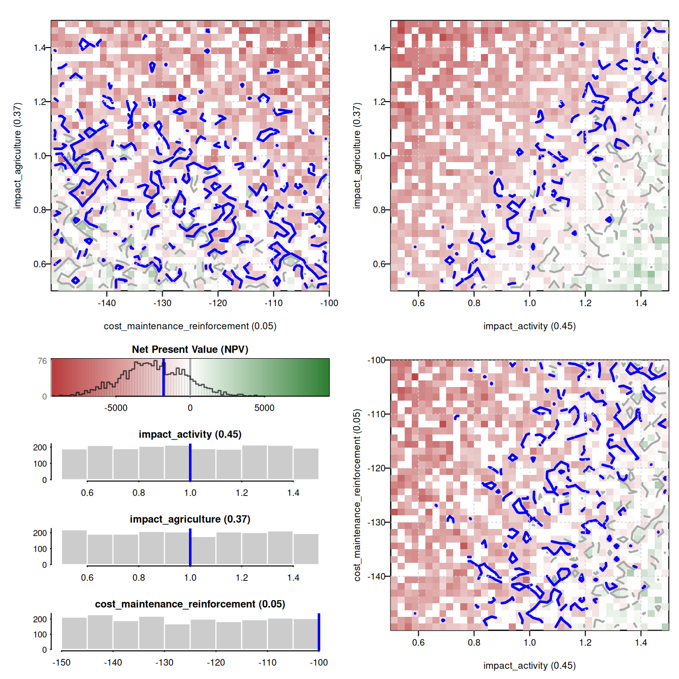
plot(sa_complete, type = "triplet")