Simulating the hydraulic behavior of the interior of a building
David Nortes Martínez and Florent Papini
hydraulic_model.RmdBasic workflow
Set up
This vignette is going to help you simulate the hydraulic behavior of
the interior of a building using floodam.building. To do so
you need 3 key inputs:
- The surface and floor level of each room
- The connections between two rooms as well as the connections with the exterior of the buildings. Hereafter we will refer to these connections as exchanges
- The evolution of the floodwater depth in front of each external wall exposed to the flood as well as the initial floodwater depth in the interior of the building (usually 0)
The library floodam.building provides methods to
calculate each of these elements. Let us see how.
To determine the two first key inputs, the function
analyse_model() provides you with the stage
hydraulic. We are using one of the models shipped with with
floodam.building to make this example:
- The models are available in your library’s installation folder. To make them available, just ask R to locate them:
#> Loading required package: floodam.building
library(floodam.building)

#> set up model to use example shipped with floodam
model_path = list(
data = system.file("extdata", package = "floodam.building"),
output = tempdir()
)-
We are going to use the model called adu_t. This model proposes a 4-room house where three of them are organized around a central living room. As stages of analysis we are going to specify
c("load", "extract", "hydraulic"). If you check the objectmodel, you can see that inside the slot called hydraulic there are four different slots containing three data.frames:- exchanges open
- exchanges_close
- exchanges_combine
- rooms
The data.frame rooms corresponds to the first key inputs, while the data.frames exchanges open, exchanges_close and exchanges_combine are variants of the second key input: all openings open, all openings closed but not waterproof, and all exterior openings closed and all interior openings open.
model = analyse_model(
  model = "adu_t",
  type = "adu",
  stage = c("load", "extract", "hydraulic"),
  verbose = FALSE,
  path = model_path
)
|
|
-
To simulate the third key input,
floodam.buildingprovides the functiongenerate_limnigraph(). This function generates a limnigraph, i.e. the evolution of floodwater depth against time. You need to manually provide different parameters to this function:- time: vector of time steps in seconds. Usually it contains three elements: the initial time step, the time step where water outside the building is at its peak, and the final time step. In the example provided this time steps are 0, 5400 and 10800 seconds.
- depth: vector of floodwater depth in meters. This vector contains as many elements as the vector of time steps. It indicated the water depth in each time step.
- external: external walls that are exposed to the flood event. In the example provided, all the external walls are assumed to be exposed to this particular flood event.
The function returns a list with a matrix named limnigraph with time steps as rows and externals as columns and an other list of externals with their walls.
flood = generate_limnigraph(
  model = model,
  time = c(0, 5400, 10800),
  depth = cbind(facade_1 = c(0, 2, 0)),
  exposition = list(
    facade_1 = list( external = c("wall_A", "wall_B", "wall_C", "wall_D",
      "wall_E", "wall_F", "wall_G", "wall_H")))
)
#> generating limnigraph ...
#>  limnigraph successfully generated
Simulate hydraulics
Once the three key parameters are determined, the simulation of the
hydraulic behavior of the building for the flood event designed can be
simulated. To do so, floodam.building provides the function
analyse_hydraulics(). This function takes three mandatory
parameters:
-
model: the output of the function
analyse_model()(see above) -
limnigraph: the output of the function
generate_limnigraph()(see above) - stage: what you want the function to perform: hydraulic, damaging, dangerosity, graph, save, display
- opening_scenario: one of the following options: open, close, combine
Additionally, the function can be provided with the parameter sim_id, in order to properly identify the simulation when working within an experimental design.
hydraulic = analyse_hydraulic(
  model = model,
  limnigraph = flood,
  opening_scenario = "close",
  stage = c("hydraulic"),
  sim_id = "integrated_model"
)
#> Simulating hydraulics for 'adu_t'...
#>  ... hydraulics successfully modeled for 'adu_t'
#> End of analysis for 'adu_t'. Total elapsed time 8.89 secs
The output of the function analyse_hydraulic() is an
object of class hydraulic. Well done! You have now successfully
processed your first hydraulic analysis. It is available inside the
object hydraulic, along with other information. Let us
explore it further.
The function returns a list of five matrices:
- evolution of floodwater depth in each room
h - evolution of the discharge volume through each opening
eQ - evolution of the discharge section through each opening
eS - evolution of the discharge velocity (calculated with the volume and
section data) through each opening
v - maximum floodwater depth in each room and their time stamp
hmax
| time | room_1 | room_2 | room_3 | room_4 | facade_1 |
|---|---|---|---|---|---|
| 0.0 | 0 | 0.0e+00 | 0 | 0 | 0.0000000 |
| 0.5 | 0 | 2.0e-07 | 0 | 0 | 0.0001852 |
| 1.0 | 0 | 4.0e-07 | 0 | 0 | 0.0003704 |
| 1.5 | 0 | 8.0e-07 | 0 | 0 | 0.0005556 |
| 2.0 | 0 | 1.5e-06 | 0 | 0 | 0.0007407 |
| 2.5 | 0 | 2.4e-06 | 0 | 0 | 0.0009259 |
| 3.0 | 0 | 3.6e-06 | 0 | 0 | 0.0011111 |
| 3.5 | 0 | 5.1e-06 | 0 | 0 | 0.0012963 |
| 4.0 | 0 | 6.9e-06 | 0 | 0 | 0.0014815 |
| 4.5 | 0 | 9.1e-06 | 0 | 0 | 0.0016667 |
We can see that the water rises in a linear fashion for
external_1. Water is flowing directly to the
room_2 because the door_1 is not waterproof.
Other rooms are filled through the indoor doors but at a very slow rate,
however knitr::kable precision is not high enough to
display numbers lower than 10E-8.
Basic visualization
floodam.building counts on methods to visualize key
information stored in hydraulic.
#> visualization of the floodwater depth
plot(hydraulic, view = "height")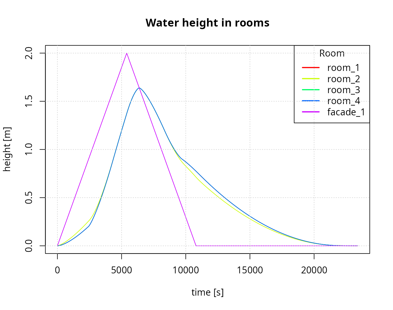
You can see that water depth is identical for room_1 room_3 room_4 due to the symetry of the building
#> visualization of the floodwater discharge in the openings
plot(hydraulic, view = "discharge")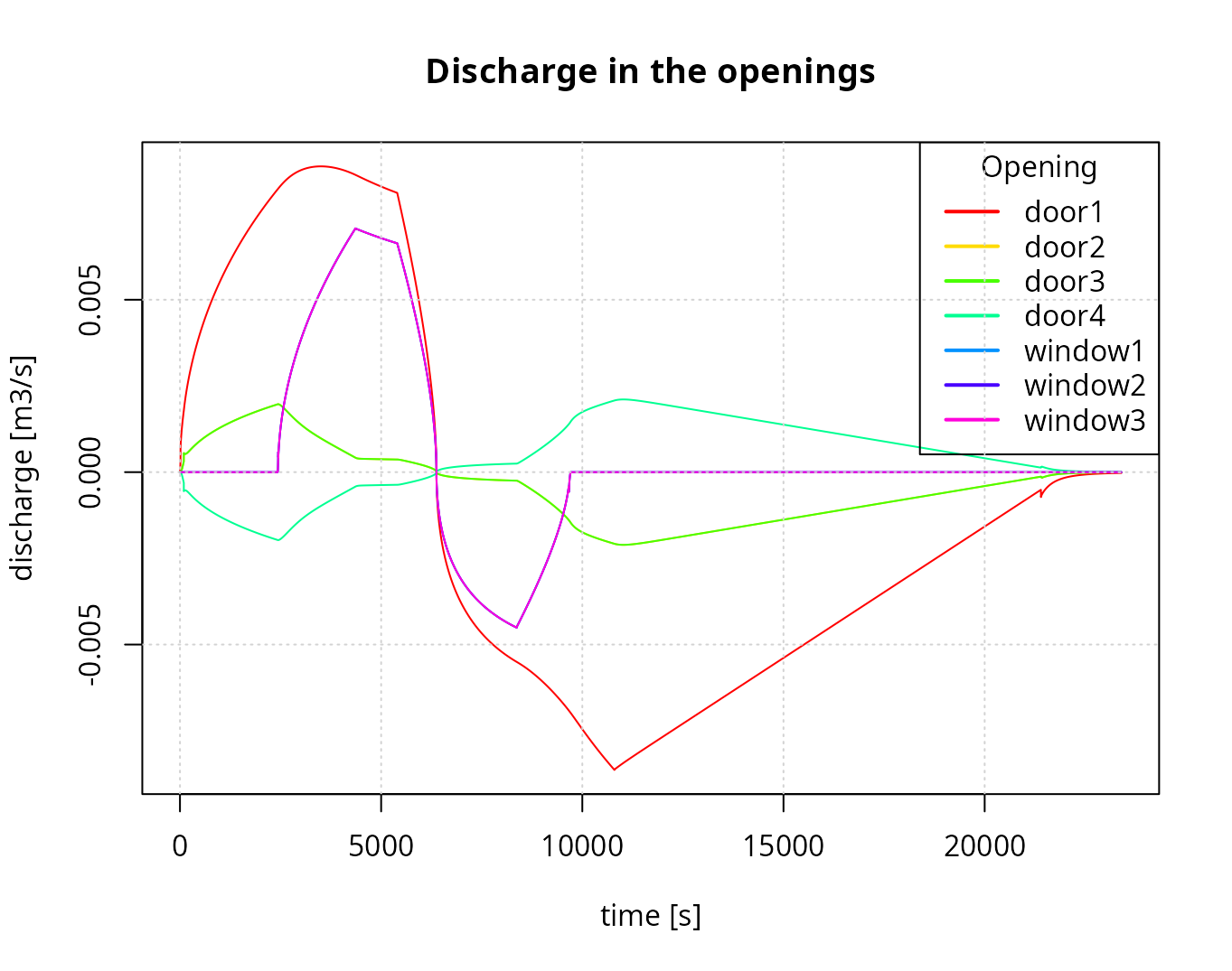
Openings are oriented, therefore you can notice either symetry or superposition for door_2 door_4 door_3, again due to the symetry of the building. If you need to know which openings are connecting the rooms you can look at this DataFrame.
| room | name |
|---|---|
| external | door1 |
| external | window1 |
| external | window2 |
| external | window3 |
| room_1 | window1 |
| room_1 | door4 |
| room_2 | door1 |
| room_2 | door2 |
| room_2 | door3 |
| room_2 | door4 |
Saving
If you are working with big simulations and don’t want to have to
rerun them you can use the stages graph and
save.
hydraulic = analyse_hydraulic(
  model = model,
  limnigraph = flood,
  opening_scenario = "close",
  stage = c("hydraulic", "graph", "save"),
  what = c("h", "eQ"),
  sim_id = "integrated_model"
)
#> Simulating hydraulics for 'adu_t'...
#>  ... hydraulics successfully modeled for 'adu_t'
#>  ... hydraulics successfully saved for 'adu_t' in '/tmp/Rtmp6hTyBv/model/adu/adu_t'
#> Plotting graphs for 'adu_t'...
#>  - Water height view save in /tmp/Rtmp6hTyBv/model/adu/adu_t/water_height.png    - Water height view save in /tmp/Rtmp6hTyBv/model/adu/adu_t/water_discharge.png
#> End of analysis for 'adu_t'. Total elapsed time 8.59 secs
graph saves in the temporary folder the basic
visualisation of water height and discharge with .png
format. The quality might be a bit low, if you need a higher resolution
you can save it in .pdf format.
#> visualization of the floodwater discharge in the openings
plot(hydraulic, view = "height", device = "pdf", output_path = model[["path"]][["model_output_hydraulic"]])
#> [1] "Water height view save in ./water_height.pdf"
save and the paramater what allows the user
to keep in the temporary folder the desired matrices stored as
.csv.gz
Multi-level dwelling
First of all, if you are working with building having multiple storeys, the object flood needs some changes.
model_basement = analyse_model(
  model = "adu_t_basement",
  type = "adu",
  stage = c("load", "extract", "hydraulic"),
  verbose = FALSE,
  path = model_path
)
# flood = generate_limnigraph(
#   time = c(0, 5400, 10800),
#   depth = cbind(external_1 = c(0, 2, 0)),
#   external = list(
#     external_1 = list(groundfloor = c("wall_A", "wall_B", "wall_C", "wall_D", "wall_E", "wall_F",
#       "wall_G", "wall_H"),
#       basement = c("wall_A", "wall_B", "wall_C", "wall_D")))
# )
hydraulic = analyse_hydraulic(
  model = model,
  limnigraph = flood,
  opening_scenario = "close",
  stage = c("hydraulic"),
  sim_id = "integrated_model"
)
#> Simulating hydraulics for 'adu_t'...
#>  ... hydraulics successfully modeled for 'adu_t'
#> End of analysis for 'adu_t'. Total elapsed time 10.86 secs
The storey name needs to be specified in the external because external walls have the same names accross storeys.
#> visualization of the floodwater depth
plot(hydraulic, view = "height")
If you’ve completed all the steps above, congratulations - the
hydraulic model has no more secrets for you. But there’s plenty of
things you can do. Let’s see what’s already implemented in
floodam.building. The next step is waiting for you here.